Recently, there seems to be an increase in image processing projects at business, and I’ve been involved in research in this field since my background in this area since my student days, I’m thrilled to be a part of these exciting projects. Raspberry Pi Image Processing OpenCV
Thus, to help you understand image processing even a little bit, I would like to perform simple image processing using the OpenCV library, which is the basics of image processing.
This guide provides an intro to using the OpenCV computer vision library on the Raspberry Pi. The guide will show you how to install and set up the library and then how to use it to perform basic image processing tasks.
By the end of this guide, you will be able to use OpenCV to load and display images, perform simple image processing tasks, and save your processed images to your machine. Checkout my last post on ESP32-CAM Object Detection Using OpenCV, Yolov3 In Python
Components Required
We require the following parts for this project. You can buy every item from the provided links:
| S.N. | Components | Quantity | Purchase Link |
|---|---|---|---|
| 1 | Raspberry Pi | 1 | Amazon | |
| 2 | Raspberry Pi Camera | 1 | Amazon | |
| 2 | SD Card 16/32 GB | 1 | Amazon | |
| 3 | 5V, 3A DC Adapter | 1 | Amazon | |
| 4 | LCD Display | 1 | Amazon | |
| 5 | Mouse & Keyboard | 1 | Amazon | |
Raspberry Pi Camera Connection
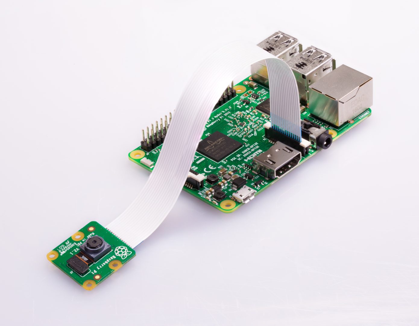
Plug the Camera Module into the Raspberry Pi 4 Board through the Camera Connector.
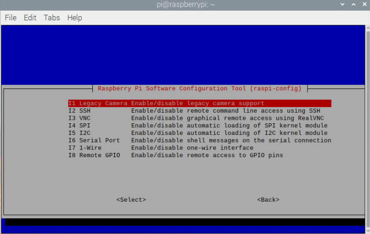
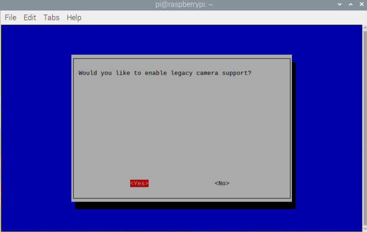
To use the camera, you’ll need to enable the Camera first. Open the Raspberry Pi Configuration Tool by typing ‘sudo raspi-config‘ in the terminal.
Then, navigate to ‘Interfacing Options’ > ‘Camera’ or ‘Legacy Camera’ and enable it. Checkout Raspberry Pi Camera Module – Setup Tutorial with Examples
Raspberry Pi Setup, Libraries Installation For Raspberry Pi Image Processing OpenCV
We’ll be using Python for image processing in this project. To get started, let’s set up the Python environment. Our key library for this task is OpenCV. Follow the following guide to install OpenCV on your Raspberry Pi system:
How to Install & Setup OpenCV on Raspberry Pi 4 -5
To verify that the library is perfectly installed, please download the image you intend to use from the following website:
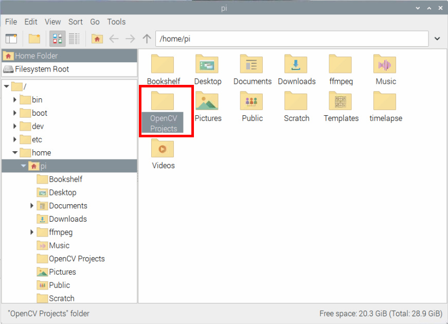
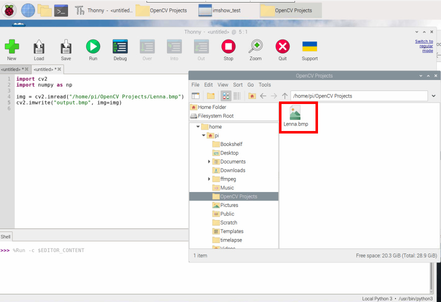
Once downloaded. Create a folder in the Home directory of your Raspberry Pi with any name such as “OpenCV Projects“. then place the image file directly within your project directory.
After that, copy and paste the below code and run it.
|
1 2 3 4 5 6 7 8 9 10 11 12 13 14 |
import cv2 import numpy as np # LOAD AN IMAGE USING 'IMREAD' img = cv2.imread("/home/pi/OpenCV Projects/Lenna.bmp") # DISPLAY cv2.imshow('imshow_test', img) cv2.waitKey(0) cv2.destroyAllWindows() |
Run the code will display the image you downloaded in a window. With this step, your preparation is now finished
Before you can start working with images, there are two important steps:
- Load the image.
- Process the image and save the result.
To load an image, you can use the code from our previous example.”
|
1 |
img = cv2.imread("/home/pi/OpenCV Projects/Lenna.bmp") |
This code will save the selected file in a variable called ‘img.’ After that, you can execute writing or processing using the following code.
|
1 |
cv2.imshow('imshow_test', img) |
Specify the file name you want to read in the ‘file name’ variable and the read image data in a variable named ‘img‘ using ‘cv2.imread.’ You can try running the following code
|
1 2 3 4 |
import cv2 import numpy as np img = cv2.imread("/home/pi/OpenCV Projects/Lenna.bmp") cv2.imwrite("output.bmp", img=img) |
When you execute this code, it will create an output file named ‘output.bmp‘ in the same location as ‘lenna.bmp.’ If you open ‘output.bmp,’ it should be an exact copy of ‘lenna_std.bmp.
Foundations of Image Processing
A pixel is a tiny dot that makes up an image on a computer screen or in a photo. Imagine a grid of these dots with different colors. Together, they create an image. A pixel is the smallest unit of image data and represents a small colored dot in an image.
For example, when you hear about Full HD, which consists of 1920 pixels horizontally and 1080 pixels vertically, these separate squares are pixels. In reality, there are 1920 squares in a row and 1080 squares in a column. Each pixel contains color data, and how this data is stored changes between color and grayscale images.
In grayscale images, each pixel is allotted a value between 0 and 255. A lower value means a darker shade and a higher value indicates a lighter shade.
In color images, each pixel has three values: one for red, one for green, and one for blue, each varying from 0 to 255. These values combine to create the colors you see in the below image.
If you’re familiar with character design in games, adjusting the RGB values for your character’s hair color follows a similar principle. You can imagine it as a grid of pixels, each holding their separate values.
Image Coordinate System
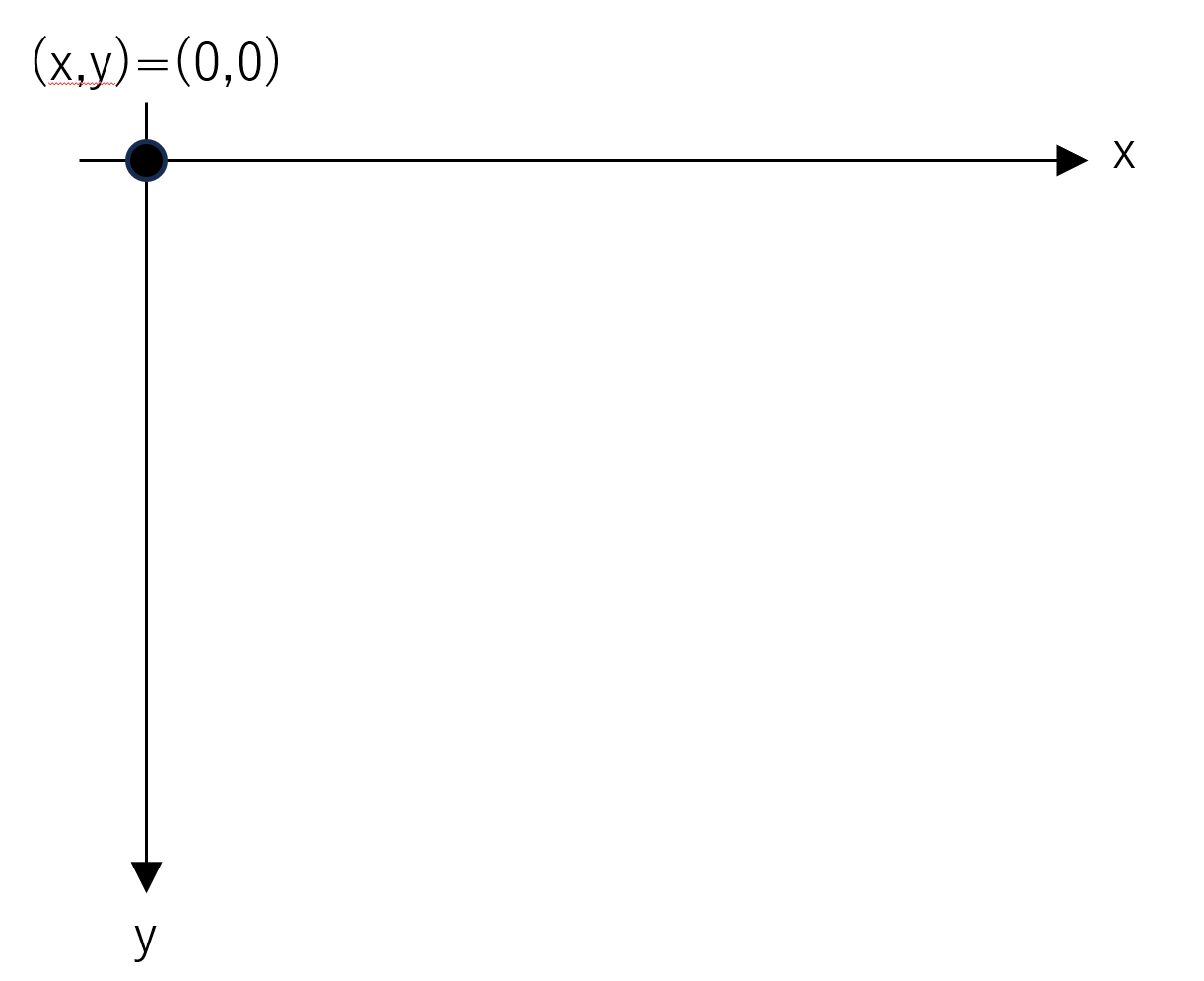
In mathematics, we usually work with a coordinate technique where the lower-left corner has coordinates (0,0), the x-value increases to the right, and the y-value increases as you go up. This is a familiar setup.
However, when working with images, the coordinate system is a bit different. In the image’s coordinate system, the x-axis remains the same (increasing from left to right), but the y-axis is flipped.
In this system, the upper-left corner of the image has coordinates (0,0), and as you move down, the y-value gets larger. It’s essential to understand this distinction to work effectively with images, so be mindful of it.”
Converting the Image to Grayscale
Now that we’ve covered the basics, it’s time to dive into using OpenCV. Our first step is to convert the image to grayscale. Here’s the code to do it
|
1 2 3 4 5 6 7 8 9 10 11 12 13 14 15 16 17 18 19 20 21 |
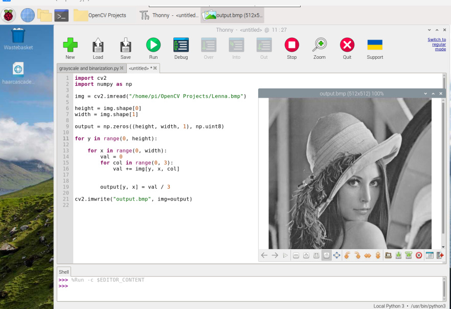
import cv2 import numpy as np img = cv2.imread("/home/pi/OpenCV Projects/Lenna.bmp") height = img.shape[0] width = img.shape[1] output = np.zeros((height, width, 1), np.uint8) for y in range(0, height): for x in range(0, width): val = 0 for col in range(0, 3): val += img[y, x, col] output[y, x] = val / 3 cv2.imwrite("output.bmp", img=output) |
The Above code will
- Load the input image.
- Get its height and width.
- Set up variables for the output image.
- For each pixel, calculate the average RGB value.
- Save the resulting image.
Running this code will transform a color image into a grayscale image, and the output will look like the image below. You’ve successfully converted a color image into grayscale!
Converting the Image into Black and White
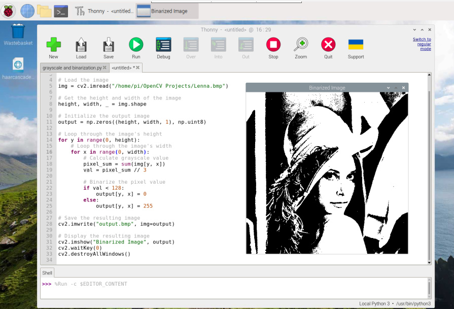
Now that we’ve successfully turned our image into grayscale, let’s take the next step and binarize it. Binarization, as the name means, simplifies the image into just two values: 0 and 255, meaning black and white. Here’s the code to perform this:”
|
1 2 3 4 5 6 7 8 9 10 11 12 13 14 15 16 17 18 19 20 21 22 23 24 25 26 27 28 29 30 31 32 33 |
import cv2 import numpy as np # Load the image img = cv2.imread("/home/pi/OpenCV Projects/Lenna.bmp") # Get the height and width of the image height, width, _ = img.shape # Initialize the output image output = np.zeros((height, width, 1), np.uint8) # Loop through the image's height for y in range(0, height): # Loop through the image's width for x in range(0, width): # Calculate grayscale value pixel_sum = sum(img[y, x]) val = pixel_sum // 3 # Binarize the pixel value if val < 128: output[y, x] = 0 else: output[y, x] = 255 # Save the resulting image cv2.imwrite("output.bmp", img=output) # Display the resulting image cv2.imshow("Binarized Image", output) cv2.waitKey(0) cv2.destroyAllWindows() |
This code follows a similar process as the grayscale conversion, but instead of using the average RGB value as-is, it separates the pixel into 0 if the average RGB value is less than 128, and 255 if it’s 128 or more. When you run the code, it makes the displayed image.
Exploring Grayscale and Binarization Using the Library
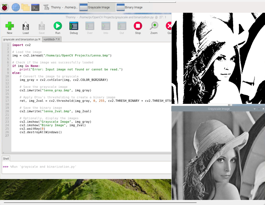
So far, we have calculated the image pixel by pixel and converted it to grayscale and binarization, but this can be done using existing libraries.
|
1 2 3 4 5 6 7 8 9 10 11 12 13 14 15 16 17 18 19 20 21 22 23 24 25 26 |
import cv2 # Load the image img = cv2.imread("/home/pi/OpenCV Projects/Lenna.bmp") # Check if the image was successfully loaded if img is None: print("Error: Input image not found or cannot be read.") else: # Convert the image to grayscale img_gray = cv2.cvtColor(img, cv2.COLOR_BGR2GRAY) # Save the grayscale image cv2.imwrite("lenna_gray.bmp", img_gray) # Apply Otsu's thresholding to create a binary image ret, img_2val = cv2.threshold(img_gray, 0, 255, cv2.THRESH_BINARY + cv2.THRESH_OTSU) # Save the binary image cv2.imwrite("lenna_2val.bmp", img_2val) # Optionally, display the images cv2.imshow("Grayscale Image", img_gray) cv2.imshow("Binary Image", img_2val) cv2.waitKey(0) cv2.destroyAllWindows() |
When you execute the above code, it will create both a grayscale and a binarized image. It’s worth noting that there are various methods for grayscale and binarization, and the output may vary from what was explained earlier.
Conclusion
In this tutorial, we explored different image processing methods as a starting point using OpenCV. I trust that this guide will be helpful for those learning on their journey in image processing

